| Home |
| Rivers - Glaciers |
| Versions |
| FAQ - References |
| Download |
| Contacts |

DASSFLOW

Estimations of the bed topography in unmonitored interior sectors of large ice-sheets: the East Antarctica case
On-going study, DassFlow version 2D shallow power-law
The computations below aim at estimating the bed topography of the ice-sheets in unobserved areas.
The physical model is valid at large scale (~30 km scale) in interior sectors (~5+-50+ m/y, milddly sheared flows).
The variational data assimilation is performed with open source or public datasets: altimetry (surface topography), Insar (surface velocities), surface mass balance (climatic data, RACMO), and airborne thickness measurements (eg Icebridge campains etc).
An example is presented below. The article [J.Monnier - J. Zhu] detailing the method and assessing it on few test cases (both in Antarctica and in Greenland) is in progress. You can see similar colorful examples on the SWOT mission website (NASA-CNES).
Goal. To derive computational methods for infering the bed elevation beneath the ice, inlands i.e. in the interior sectors of the ice sheets where no airborne measurement is available (or at best very few).
Where ? Wherever beneath the ice-sheets (Antarctica, Greenland) where the ice surface velocity ranges from ~5+ to 50+ m/year.
What data are available ?
Surface velocities (InSAR), surface elevation (altimetry e.g. ESA-Cryosat 2, SWOT etc) and airborne thickness measurements (e.g. from Nasa IceBridge campains). Our "first guess" is the currently most accurate estimation that is BedMap2 [Fretwell et al.] (see below).
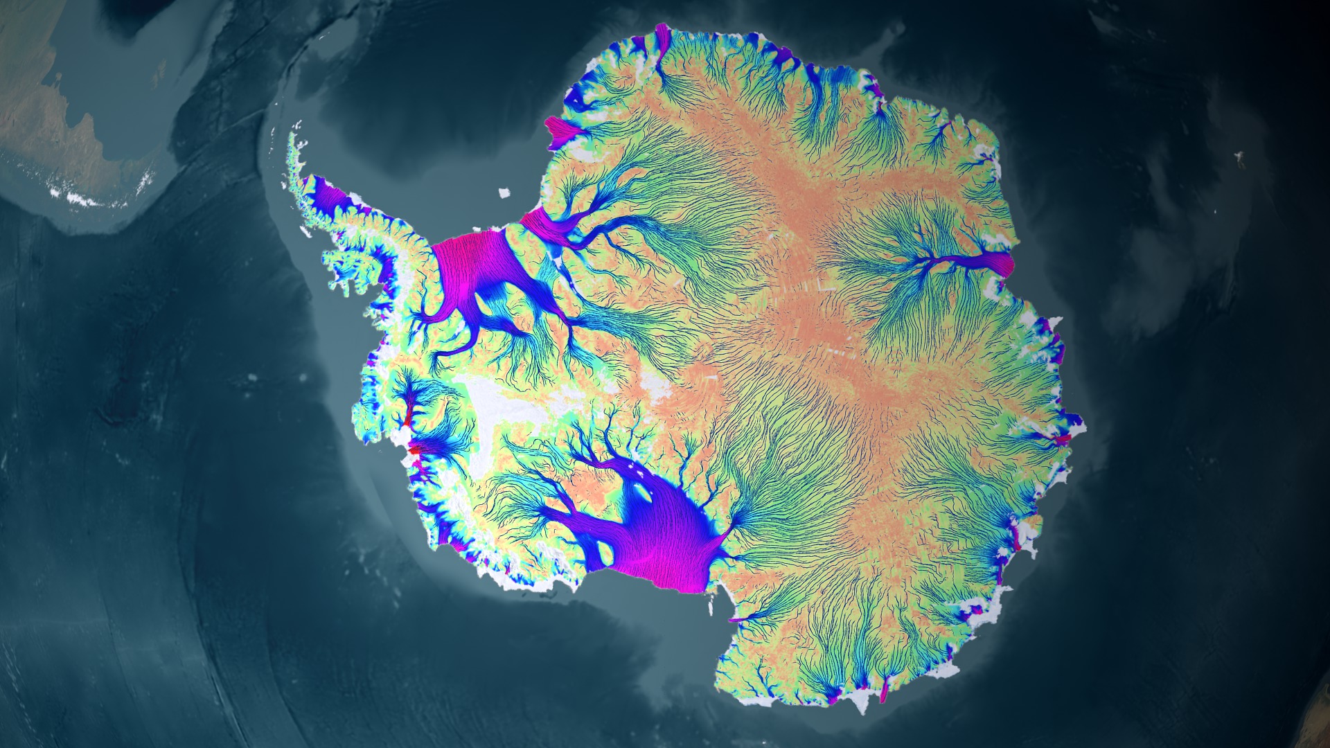
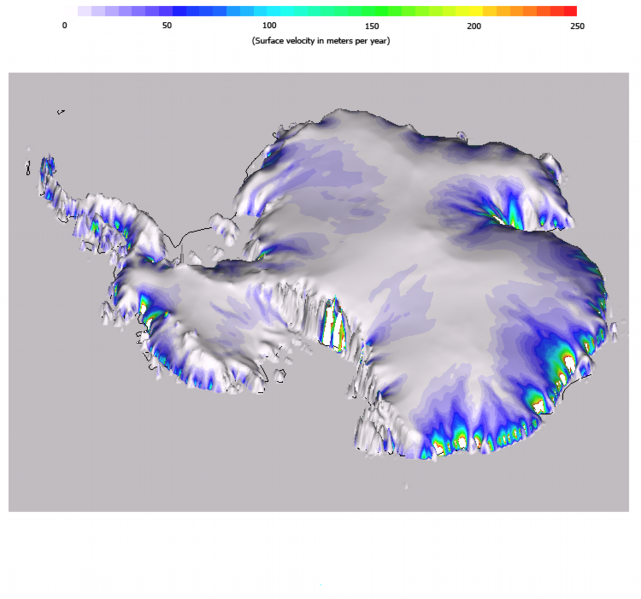
Figures: Antarctica. (L) Surface velocity from CSA, JAXA and ESA, processed by the glaciology group from UC Irvine, California. (Fine resolution). (R) Surface velocity combined with the surface elevation. (Image source: Community Ice Sheet Model website; coarse resolution). |
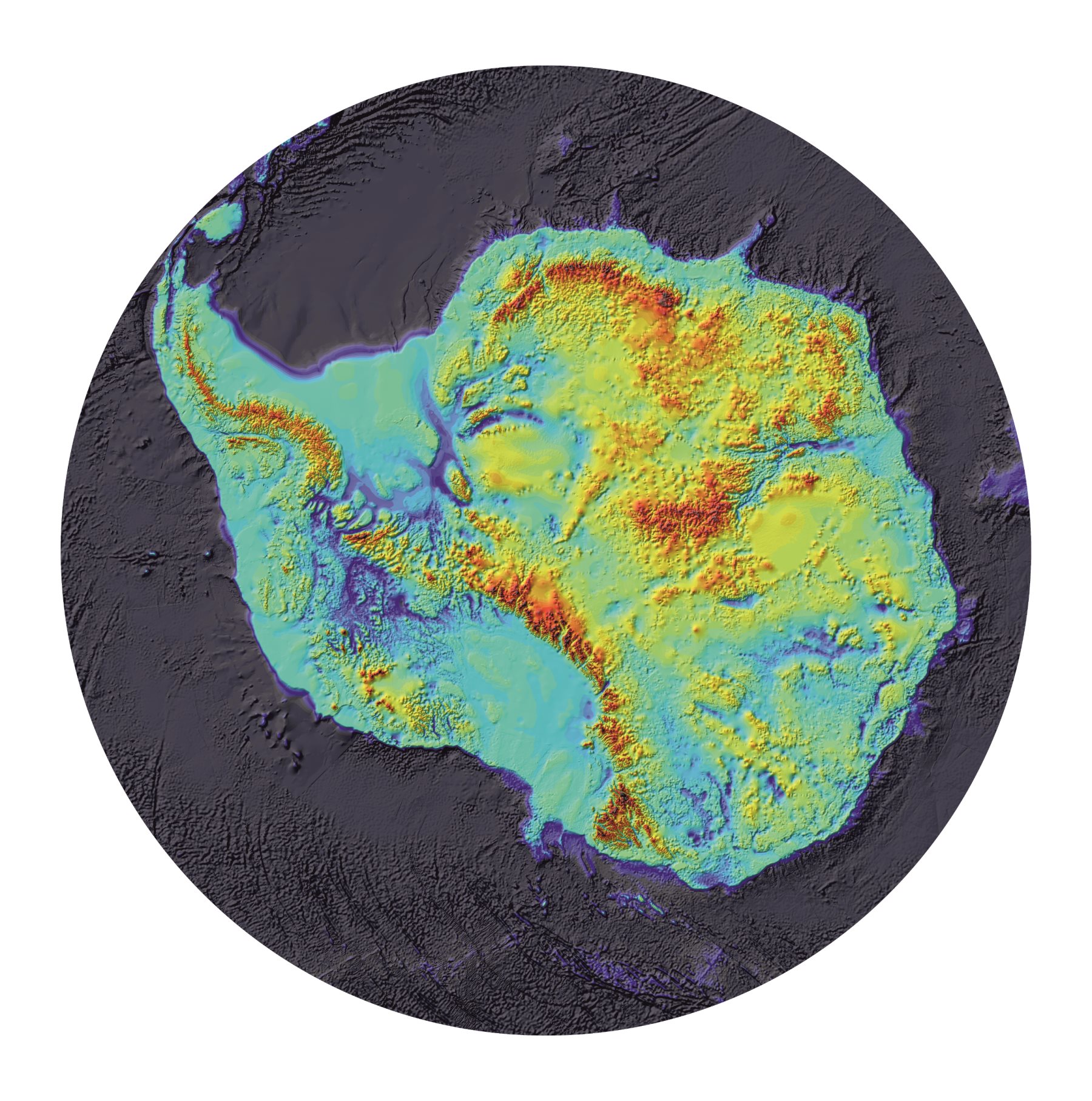
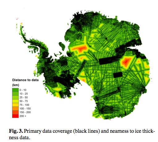
Figures: Antarctica bed topography: Bedmap2. Ref. Fretwell et al., 2013. International dataset, map produced by British Antarctic Survey (BAS), UK. (L) Bed elevation beneath the ice, measured or estimated. In interior sectors: estimations computed e.g. by krigging or gravimetry. (R) Distances to the acquired data.
What are the ingredients of our computational method ? A so-called "Reduced Uncertainty formulation" of the full physics (mass, momentum, thermal) under the long wave assumption (shallow flow model) and an advanced variational data assimilation process (taking into account a-priori uncertainties and physical lenght scales) + pseudo-analytic uncertainties quantification.
What do we obtain ?
- In Greenland unmonitored areas: bed bathymetry elevations quite similar to the current estimations (obtained by simple kriging interpolation): ~3% of differences). This confirms the current estimations in these relatively small unmonitored areas (the physical based model is large scale and the airborne measurements are quite dense now on this continent).
- In large unmonitored areas of Antartica (inland where Us range from 10 to 80+m/y). We obtain new estimations of the bed elevation with uncertainties greatly smaller than the present ones: uncertainties of ~200m instead of ~1000m or ~350m depending on the considered areas.
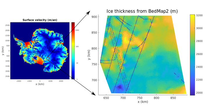
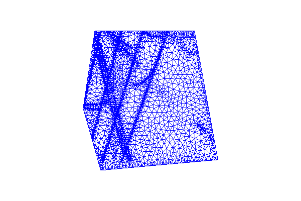
Figures. (Left) DassFlow computations on an Antarctica portion (a ~200x200 km portion for a sake of readability).
(Right) A (coarse) numerical grid to solve our mathematical systems; the flights tracks with tickness measurements are easily notable.
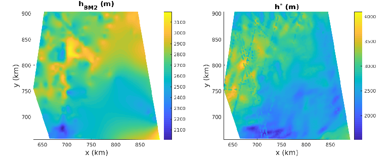
Figures. (Left) The ice thickness (m) estimated in BedMap2 (Fretwell et al., British Antartica Survey, UK) (= our first guess).
(Right) The ice thickness (m) estimated by our physical-based model (mean difference of ~218m ~ 8% with BedMap2).
Computations IMT-INSA 2018, J. Zhu. Articles under preparation.