Clinical dynamic SPECT movies (based on self-experiments)

Dominikus Noll

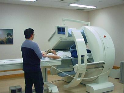
In dynamic SPECT with a slowly rotating SPECT camera, data are obtained by a standard clinical acquisition protocol.
That means for instance, 20 - 30 minutes, during which the camera performs a 180 degree rotation, taking 60 views.
The difference between dSPECT and the traditional clinical SPECT is that the tracer is dynamic, which means due to
rapid uptake and washout in the body, activity in the organ changes significantly during these 20-30 minutes.

Mathematically, in SPECT, we reconstruct an unknown emission source f(x) which varies spatially, x ∈ R³. Projection
data are of the form

(1)      p(⋅,t) = R_t[μ] f(⋅)

(2)      p(⋅,t) = R_t[μ] f(⋅,t).

In other words, as the camera goes from angular position φ to φ+Δφ, and time goes from t to t+Δ t, the source f(x,t) has
evolved from f(x,t) to f(x,t+Δ t), and has therefore changed significantly. The data p(s,t) are called sinogram, and can be
visualized as a movie. Here is the case of a kidney acquisition.

kidney_sinogram.mpg

You have the feeling that the camera rotates around the patient. For myocarial SPECT this looks much more noisy.

heart_sinogram.mpg

You understand why cardiologists refer to the heart as a donut. Watching the movie p(s,t), (s ∈ R² pixel of the camera),
we have to be aware that there is a fundamental difference with a standard movie (like Dr. Shiwago), where a 3D+time
quantity is displayed as 2D+time. The sinogram is only 2D+time, displayed as such. In other words, you might believe
perceiving a spatial object, around which you rotate, but there is none, only 2D+time.

Inverting (2) is much harder than inverting (1). The mathematical model of (1) is based on the photon transport equation.
To invert (2), you need to complete this by a mathematical model of the tracer kinetics. The inversion can then no longer
be based on integral geometry (like filtered backprojection) or on versions of the EM-algorithm (like OSEM). Instead, we
need nonlinear optimization techniques to reconstruct f(x,t). You may check my publications to get more information on
the reconstruction technique. We are holding a patent for this slow rotating reconstruction method.

Let us look at some reconstructions based on data like the kidney sinogram. Notice that we are now displaying a 4D
quantity f(x,t). The first movie is surface rendered. Notice that a study of approximately 20 minutes is visualized.

kidney_surface_rendered.mpg

The isosurface of constant activity shrinks into the interior of the organ, because the tracer is washed out into the bladder.
This gives the impression that the organ shrinks. The ureter shows up after some delay, while it is initially absent, as there
is no activity. This is interesting, yet certainly not the way doctors would like to see the reconstruction. The following is
also surface rendered.

hot_kidney1.mpg
hot_kidney2.mpg       renal.avi

Interestingly, one of the ureters does not show up in the reconstruction. This does not mean the test person does not have it,
but that is was carrying significantly lower activity, so that the thresholding gave it 0 value.

The following two movies show a representation by partial volume rendering. You can see the hot zone inside the organ
and can notice the change of activity. The rotation around the object is created for the convenience of the observer.

partially_volume_rendered1.mpg
partially_volume_rendered2.mpg
ideally_volume_rendered.mpg

Doctors would typically prefer to see the organ reconstruction trace-by-trace. That would be as follows.

These images represent results of self-experiments performed at the Vancouver General Hospital in cooperation between
my team and the team of Anna Celler. We also used phantoms to test our reconstruction techniques. That could look as
follows.

hot_bottles1.mpg
hot_bottles2.mpg
surface_rendered_bottles.mpg

In (2) one assumes the attenuation map μ(x) known. This is usually possible if the dSPECT study is combined with a
transmission study (like a CT). But mathematicians have also tried to invert the operator (μ,f) → R[μ] f simultaneously.
F. Natterer has contributed to this line, and so has my team in cooperation with J.-P. Esquerré from Purpan Hospital in
Toulouse. This is a difficult non-linear ill-posed inverse problem. See e.g. the following paper: