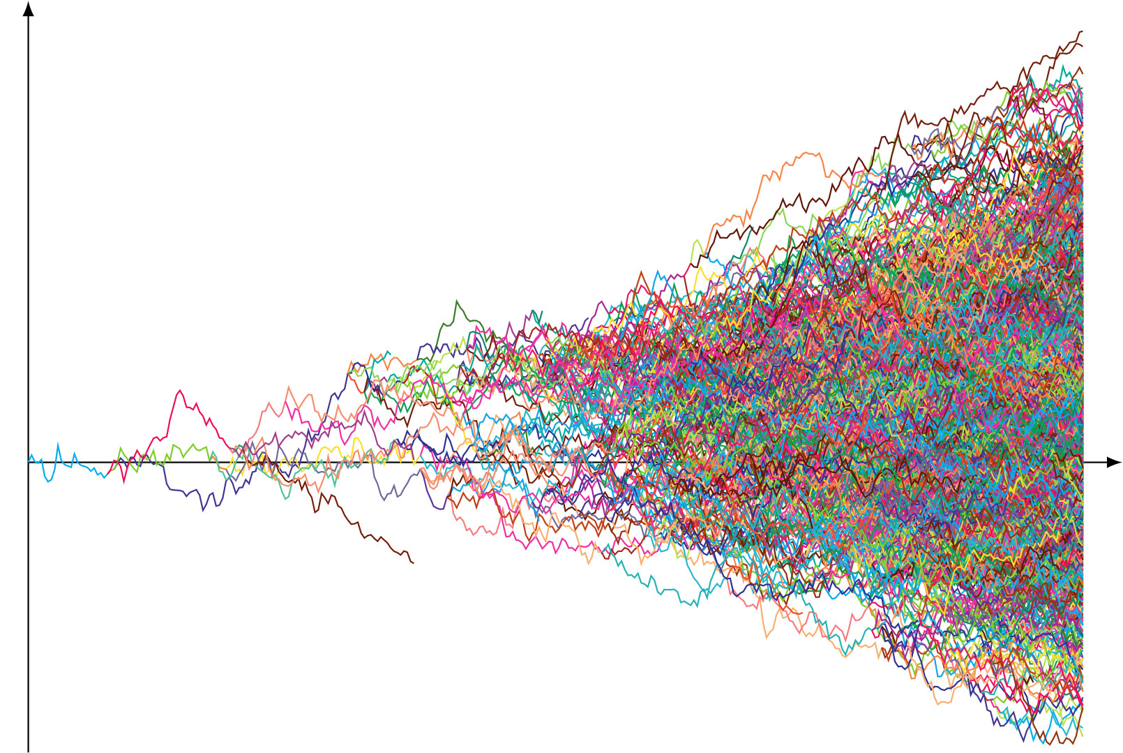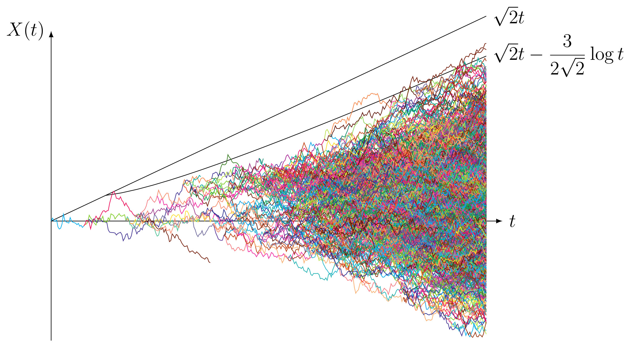
Standard branching Brownian motion

Initially, there is one particle at the origin. It moves as a Brownian motion and, after an exponentially distributed time, it dies, giving birth to two children. These children start from its position and moves as independent Brownian motions during independent exponentially distributed times and then die, each giving birth to two children. And so on.

One can replace the binary splitting by a random reproduction: when a particle dies, it gives birth to a random number of children chosen according to a given reproduction law. For example, in the branching Brownian motion below, each particle has 0 child with probability 15%, 2 children with probability 65%, 3 children with probability 10% and 4 children with probability 10%. Hence, the mean umber of children is still 2. A vectorized version of this picture is available here.

Position of extremal particles

A main focus on branching Brownian motion has been the study of the position of the highest particle at a given time. At first order, branching Brownian motion behaves like a cone and the highest particle moves at speed \(\sqrt{2}\). More precisely, the position of the highest particle at time \(t\) is asymptotically given by \[\sqrt{2}t - \frac{3 \log t}{2 \sqrt{2}} + O(1),\] and Bramson proved the \(O(1)\) term converges in distribution.