Mandelbrot set
Here we will give a few algorithms and show the corresponding results.
Contents
The Mandelbrot set
Certainly, Wikipedia's page about this set in any language should be a very good introduction to this set. Here I give a very quick definition/reminder:
The Mandelbrot set, denoted M, is the set of complex numbers $c$ such that the critical point $z=0$ of the polynomial $P(z)=z^2+c$ has an orbit that is not attracted to infinity. If you do not know any of the italicized words, go and look on the Internet.
It is interesting for two reasons:
- The Julia set of $P$ is connected if and only if $c\in M$.
- The dynamical system $z\mapsto P(z)$ is stable under a perturbation of $P$ if and only if $c\in \partial M$, where $\partial $ is a notation for the topological boundary.
Drawing algorithms
All the algorithms I will present here are scanline methods.
Basic algorithm
The most basic is the following, it is based on the following theorem:
Theorem: The orbit 0 tends to infinity if and only if at some point it has modulus >2.
This theorem is specific to $z\mapsto z^2+c$, but can be adapted to other families of polynomials by changing the threshold $2$ to another one. Here the threshold does not depend $c$ but in other families it may.
Now here is the algorithm:
Choose a maximal iteration number N
For each pixel p of the image:
  Let c be the complex number represented by p
  Let z be a complex variable
  Set z to 0
  Do the following N times:
    If |z|>2 then color the pixel white, end this loop prematurely, go to the next pixel
    Otherwise replace z by z*z+c
  When the loop above reached its natural end: color the pixel p in black
  Go to the next pixel
I am not going to use the syntax above again, since it is too detailed. Let us see what it gives in a Python-like style:
for p in allpixels:
  complex c = p.affix
  complex z = 0
  color = black # this color will be assigned to p at the end, black is a temporary value
  for n in range(0,N):
    if squared_modulus(z)>4:
      color = white
      break: # this will break the innermost for loop and jump just after
    z = z*z+c
  p.color = color # so it will be white unless we ran into the line color=black
Here in a C++ like style: (std::complex<double> simplified into complex)
for(int j=0; j<height; j++) {
  for(int i=0; i<width; i++) {
    complex c = some formula of i and j;
    complex z = 0.;
    for(int n=0; n<N; n++) {
      if(squared_modulus(z)>4) {
        image[i][j]=black;
        goto label;
      }
      z = z*z+c;
    }
    image[i][j]=white;
    label: {}
  }
}
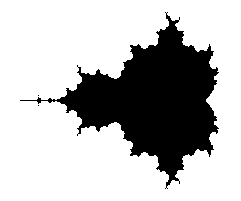
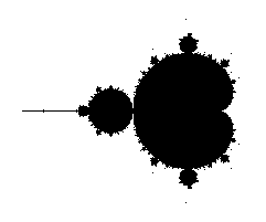
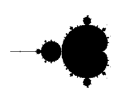
Let us now look at the kind of pictures we get with that. We an image size of 241x201 pixels, with a mathematical width of 3.0 and so that the center pixel has affix -0.75. The only varying parameter between them is the maximal number of iterations N.
N=10

N=20
N=100
N=1 000 000


All images except the last one took a fraction of a second to compute on a modern laptop. Back then in the 1980's it was different.
Ideally the maximal number of iterations N should be infinity, but then the computation would never stop. The idea is then that the bigger N is, the more accurate the picture should be.
The N=one million image took 45s to compute on the same laptop, which is pretty long given today's computers power. What happens? Every black pixel requires $10^6$ iterations, and since there are 9 771 of them, we do at least ~$10^10$ times the computation z*z+c. To accelerate this, one should find a way to detect that we are in M so that we use less than the maximal number of iterations.
But that is not the only problem with increasing N. Not only it took much time, but the difference with N=100 is pretty small. Worse: it seems that by increasing N we are losing parts of the picture. What happens is that we are testing pixel centers or corners, and there are strands of M that are thin and wiggle between the pixel centers, so that as soon as N is big enough, the pixel gets colored white.
Here are enlarged versions of parts of these images, so that pixels are visible.


Let us look at a parts of a higher resolution image, computed with a big value of N: notice the small islands. The set M is connected in fact, but the strands connecting the different black parts are invisible, except some horizontal line that appears because, by coincidence, we are testing there complex numbers that belong to the real line: $M\cap \mathbb{R} = [-2,0.5]$.

The next image has been computed using a 4801x4001 px image and then downscaling by a factor of 6 (in both directions) to get an antialiased grayscale image. It also has been cropped down a little bit, to fit in this column without further rescaling.

Last, an enlargment to see the pixels of the above image:

Escape time based coloring
There is a simple and surprisingly efficient modification of the above algorithm.
We started from z=0 and iterated the substitution $z\mapsto z^2+c$ until either |z|>2 (the orbit escapes) or the number of iterations became too big. Instead of coloring white the pixels for which the orbit escapes, we assign a color that depends on n, the first iteration number for which |z|>2.
For the coloring, you are free to take your preferred function of n, I will not develop on that here.
Here is an example of result:

The strands became visible again.
Here is another one, on a 4801x4001 px grid, downscaled by a factor 5, with N=10000 (which is probably a bit excessive).

With a nicely chosen color function, one can get pretty results:

The following was popular in printed books:

The potential
You may replace the test |z|>2 by |z|>R, provided that R>2. In fact the picture looks better that way. It has an explanation in terms of the potential.

In very informal terms, in a 2D euclidean universe, put an electrostatic charge one on some bounded connected set K. The charges move to minimize the energy, and the resulting distribution has the property that the potential is constant on K. The potential function $V$ satisfies the Laplace equation $\Delta V=0$ outside K and $V(c)\sim \rho \log|c| $ when $|c|\longrightarrow+\infty$.
There is however no need to invoke electrostatics and one can define directly the following function and decide to call it "potential": $$V(c)=\lim_{n\to+\infty} \frac{\log_+|P_c^n(0)|}{2^n}$$ where $\log_+(x)$ is defined as $0$ if $x<1$ and $\log(x)$ otherwise. The exponent n in $P_c^n$ refers to composition, not exponentiation: $P^n(z)$ is P applied n times to z. The function V takes value 0 exactly on M. If x>0, the sets of equation V=x are called equipotentials of M. They are smooth simple closed curves that encircle M.
The fact that the formula converges and that its limit has the stated properties is not supposed to be obvious: it is a theorem. One good thing about the formula is that it converges quite well: if we stop the iteration when |z|>R, the relative error will be of order 1/R. Now assume the picture is drawn for $|c|<10$ (anyway all points of M satisfy $|c|\leq 2$) and at some point in the iteration of $0$ we reach $|z|>4$. Then a value of $|z|>1000$ is reached pretty fast because $P(z)=z^2+c>|z|^2-5$: one sees that in 4 more iterations we have at least |z|>443556...