A generalization of the Linear Quadratic Gaussian Loop Transfer Recovery procedure (LQG/LTR)
Dominikus Noll
Key words. Kalman filter. Apollo program. Lack of robustness of LQG. Heuristic LTR procedure to robustify LQG. Failure of LTR. How LTR can be safed and turned into a mathematically sound approach.
Contents
The 1960s. Kalman filter and the Apollo program
Linear Quadratic Gaussian (LQG) control dates back to the work of E. Kalman in the 1960s. Its potential was recognized by the Apollo people, and the Kalman filter became the first embedded system.

Fig. 1. Bord computer of Apollo 8, containing the Kalman filter
LQG is based on the so-called principle of separation of control and estimation. The state-feedback controller K is optimal in the sense of a quadratic criterion, and the Kalman filter K
 is the optimal state estimator in the presence of white noise disturbances. Taken together controller and filter give a control law which is optimal in the presence of white noise measurement and process noise.
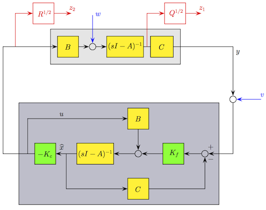
Fig. 2. Observer-based controller. Inputs are process noise w and measurement noise v. Controlled outputs are weighted x and u. Elements to be synthesized in green.
The 1970s. Lack of robustness
The enthousiam about LQG was damped by several spectacular failures of the method in practical situations. In 1975 the LQG controller for a Trident submarine caused the vessel to unexpectedly surface in a simulation of rough sea, and the same year LQG control of the F-8C crusader aircraft led to disappointing results. It became apparent that LQG lacks robustness to system uncertainty. A change of paradigm was needed. George Zames posed the problem of robust control, also known as H -synthesis. This problem was solved 30 years later in 2004 by P. Apkarian and D. Noll [1,2]. Since 2010 the solution is available to the control community via the functions hinfstruct and looptune of the Robust Control Toolbox.
doc hinfstruct; %doc looptune;
A remedy: Loop transfer recovery
LQG/LTR is a heuristic remedy to the lack of robustness of LQG. It was first proposed by H. Kwakernaak [3], and later popularized by Stein, Athans and Doyle in a series of papers [4-6]. Its basic idea is as follows. Let P be the plant of Figure 2 above. Create a one-parameter family P( ) of modified plants such that P = P(1) is nominal, and for -> 0, the closed-loop output sensitivity function S = inv(I+GK()) approaches the target sensitivity function S
 of the state-feedback controller. In other words, the sensitivity of the controller K() is reduced, either by artificially increasing the noise level at the output y (via ), or by artificially increasing the LQG-cost via a parameter q, where Q(q) = Q + qC'C.
What goes wrong in LQG/LTR ?
The LQG/LTR procedure increases the robustness of the design (by de-sensibilizing). But there is a price to pay. The original LQG cost degrades. In other words, the performance of the closed-loop system degrades significantly. This can be seen in the following
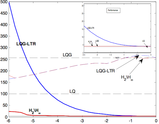
Fig. 3. As the noise level is artificially increased ( -> 0), the  -norm of the sensitivity function S (dashed magenta) decreases and approches the dashed horizontal line labeled LQ, the target sensitivity function of LQ. Since the latter has optimal robustness, overall robustness of the design is enhanced. However, the original performance is degraded (blue line goes to infinity as -> 0). This failure can be remedied by the procedure we have developed (red line). See [7,8] for details.
2009. The new idea.
The new idea was first presented by D. Noll in a plenary talk at the 2009 French-German conference on optimization in Leuven. It is as follows (see [8,9]): If the nominal LQG-controller K(1) lacks robustness, we choose 0 < < 1 such that the modified LQG controller K() is less sensitive, and therefore sufficiently robust in the sense that S() =  inv(I + K()G)
  = r() is small enough. Since this controller will have a degraded performance, we solve the mixed
  -optimization program
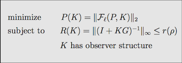
Fig. 4. The mixed -synthesis program.
This leads to a controller K  () which has the same robustness as K(), but strikingly better LQG-performance, as seen in Fig. 3 (red curve versus blue curve). It requires being able to solve a mixed -synthesis program with a given structure, here the observer structure. The first algorithmic approach which makes structured mixed synthesis possible was presented in [9] and is based on non-smooth optimization techniques. Notice that neither ltrsyn nor hinfmix allow to do this. They provide full-order controllers, and do not lead to the observer structure.
| LQG/LTR | New method | |
| advantage | easy to use | good robustness and performance |
| disadvantage | degraded performance | needs code for optimization |
Fig 5. Advantages and disadvantages of both methods.
Limitations
One should notice that LTR does not work for non-minimum phase systems G. Our mixed synthesis program of Fig. 4, on the other hand, may still be applied as is, with the difference that LTR can no longer be used to calibrate the procedure. However, it may be advisable to replace the sensitivity function by a filtered version, see remark 8 in [7] for indications how to proceed.
Extensions beyond observer-based controllers
In [7,8] we have shown how the same approach can be extended to other more practical controller structures like PIDs. The structured mixed program can still be solved using our code [9]. However, finding the robustness level r() can no longer be based on LTR, and a substitute must be found. This calibration can be obtained as follows. Having a nominal controller K(1) which is not sufficiently robust, its robustness gives an upper bound ru. To get a lower bound we solve the unconstrained structured optimization program
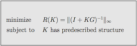
Fig 6. Use structured -synthesis [1] to calibrate. This problem is non-convex.
using hinfstruct based on [1,2]. This leads to the most robust controller K of the given structure and gives a lower bound rl for the sensitivity constraint. The final step is to locate an appropriate intermediate value rl < r < ru, where a compromise between robustness and performance is achieved, by solving the structured mixed -program again.
Visualization in 2D
Suppose we start by synthesizing an LQG controller. As this is a linear quadratic problem, we visualize this by a quadratic optimization problem in 2D. You can imagine that there are two unknown controller gains to be computed, so every point in the plane is a candidate. The one which minimizes the LQG criterion is the black dot. The ellipses are the level curves of the LQG objective. Notice that the problem is convex.
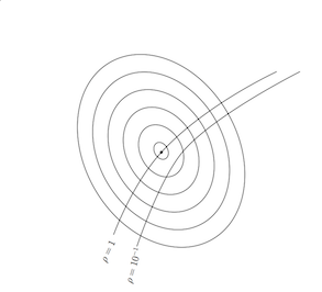
Fig. 7. Nominal synthesis, lacking robustness.
Now our working hypothesis is that the LQG controller is not sufficiently robust. In the plot its robustness is the curve  . But suppose we need at least robustness
  , the second curve. See what the LQG/LTR procedure does.
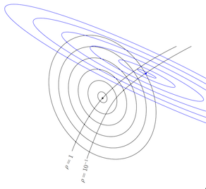
Fig. 8. Deformed LTR synthesis gives better robustness.
It deforms the nominal LQG problem into an artificial one, now indicated by the blue lines. The optimal controller for this problem is now the blue dot, and it has the desired robustness, as it lies on the curve . Notice that the level curves are still ellipses. The blue dot, representing the LTR-controller for , is still easy to compute. Suppose we need even more robustness, say  . This is what happens:
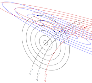
Fig. 9. Further deformed is even more robust.
The problem is further deformed, the LTR-controller for is now the red dot. As you can see, the deformation with parameter gives a 1-parameter family of controllers, visualized by the magenta curve in Fig. 10 below. As we go from the black dot through the blue dot to the red dot, we increase robustness from  to and then .
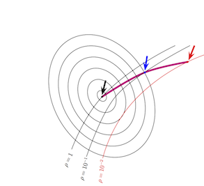
Fig. 10. LTR-controller  as a 1-parameter family.
Unfortunately, this leads to a dramatic loss of performance. The big black ellipse gives the level curve on which the red dot lies with regard to the original LQG problem. We have strongly degraded performance with regard to the original LQG problem.
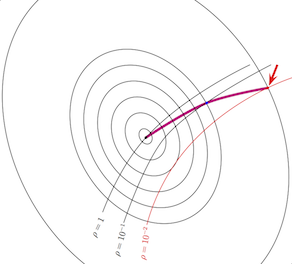
Fig. 11. Loss of performance is significant.
This is where our new procedure sets in. We solve the constrained optimization problem in Fig. 4, where the original LQG objective P(K) is minimized subject to a robustness constraint R(K) <= R(K()). This means we are as robust as LTR-controller on the curve, but achieve a way better preformance with regard to the original problem. The new controller is visualized by the green dot where the line touches the level curve of the original optimization problem.
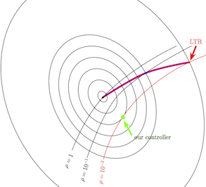
Fig. 12. Green dot is constrained minimum of -program.
The gain in perfomance is evident. In exchange, the improved LTR-controller is harder to compute. It is no longer an LQG controller of any kind, so in particular, there is no longer any separation principle, and there are no Riccati equations to compute it. Yet, the new controller still has observer structure, because we imposed this as a constraint. What you need to do this is nonlinear optimization.
Alternatives
Professional software implementing -synthesis is currently under development and is based on the seminal work [1,2,9]. The difficulties lie in the non-smoothness of the robustness constraint, which uses the -norm. However, one can robustify LQG using smooth optimization only. How this can be done is explained in my tutorial on parametric robust H2 control.
References
[1] P. Apkarian, D. Noll (2006). Nonsmooth H infinity synthesis. IEEE TAC,AC-51:71-86.
[2] P. Apkarian, D. Noll (2006). Nonsmooth optimization for multidisk H-synthesis. European J. Control,12(3):229-244
[3] H. Kwakernaak (1969). Optimal low-sensitivity linear feedback systems. Automatica,5:279-285.
[4] G. Stein, M. Athans (1987). The LQG-LTR procedure for multivariable feedback control design. IEEE TAC, AC-32:105-114.
[5] J. Doyle, G. Stein (1981). Multivariable feedback design: concepts for a classical/modern synthesis. IEEE Trans. Autom. Contr. AC-26:607-611.|
[6] M. Athans (1986). A tutorial on the LQG/LTR method. Proc. Amer. Control. Conf. Seattle.
[7] L. Ravanbod, D. Noll, P. Apkarian. An extension of the linear quadratic Gaussian loop transfer recovery procedure. IET Control Theory and Applications 2012.
[8] L. Ravanbod, D. Noll, P. Apkarian (2011). On a generalization of the LTR procedure. CCDC 2011:2634-2639.
[9] P. Apkarian, D. Noll, A. Rondepiere (2008). Mixed H2/Hinfinity control via nonsmooth optimization. SIAM J. Control Optim. 47(3):1516-1546.