The H_∞ control problem is solved

by

Pierre Apkarian and Dominikus Noll

Abstract.
The

H_{∞}

-control problem was stated in the 1960s by George Zames and finally solved by
Apkarian and Noll in 2006. The Matlab function hinfstruct based on work of Apkarian,
Noll and Gahinet 2006 - 2010 makes the mathematical solution available to the control
community.

What is the rationale of $H_{∞}$ -control?
Milestones to the solution 1960 - 2006.
How to use hinfstruct in practice

Rationale.
The

H_{∞}

control problem can be cast as follows. Given a proper transfer operator

P (s)

and
a set

K of proper controllers

K (s)

, find

K^{*}

∈ K which stabilizes

P

internally such that

the

H_{\infty}

-norm of the closed-loop transfer function

T_{wz} (K^{*}, s)

from

w

z

is minimized at

K^{*}

among all internally stabilizing controllers

K

∈ K. In other words,

K^{*}

is an optimal solution
of the optimization program

minimize

| | T_{wz} (K) | |_{∞}

subject to

K

stabilizes

P

internally (1)

K \in K

where

z (s) = T_{wz} (K, s) w (s)

is the response

z

of the closed-loop system to input

w

when
controller

K

is used, and the

H_{∞}

-norm is nothing else but the

L^{2} - L^{2}

operator norm. As
we shall see, the crucial question in (1) is how to choose the space K.

Milestones
The famous 1989 paper by Doyle, Glover, Kargonekar and Francis gives a solution of
the

H_{∞}

control problem (1) when K is the space of all controllers

K

having a state-space
realization

(A_{K}, B_{K}, C_{K}, D_{K})

with the same order as the plant

P

. That is, the size of

A_{K}

is the
same as size of the

A

-matrix in the plant

P

. This is the largest possible class K. It leads to
the famous characterization of the central

H_{∞}

-controller by 2 decoupled algebraic Riccati
equations. The Matlab function hinfric uses this approach.

Another milestone is the 1995 discovery by Gahinet and Apkarian that the

H_{∞}

probem
over the same largest class K of full-order controllers could also be transformed into a
linear matrix inequality (LMI) and solved as such. This approach is used in the Matlab
function hinflmi.

Using structured $H_{∞}$ control
The 1-degree-of-freedom control (1-DOF) is a simple set-up to demonstrate the use
of

H_{∞}

-control. In the scheme below red arrows represent inputs to the closed-loop
system like reference signals

r

, process noise

n_{p}

, disturbances

d

, and sensor noise

n_{s}

.
The blue arrows are controlled outputs in closed-loop, which we typically want to be
small. For instance,

e

on the left is the tracking error, and ê is a filtered version of

e

,
where

W_{e}

is typically a low-pass filter. In contrast,

W_{u}

might typically be a high-pass
filter, penalizing high frequency control action.

Given the performance channel

w \to z

with

w = (r, n_{p}, n_{s})

and

z = (W_{e} e, W_{u} u, W_{y} y)

,
we seek

K \in

K

An example of a structured controller
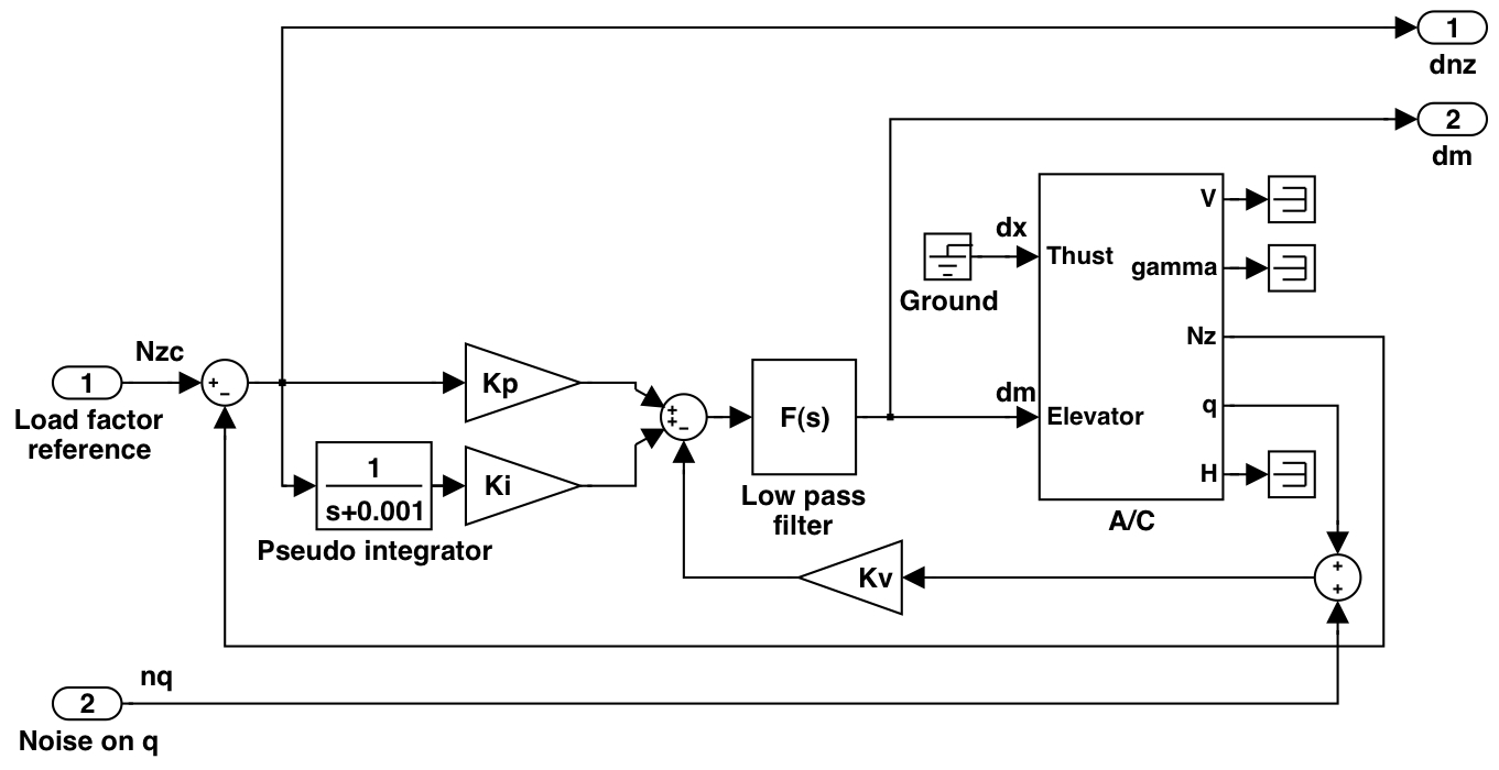
We consider the flight control loop in longitudinal control of an aircraft. The following
scheme shows the situation, where the flight controller has to generate the elevator
deflection

d m

, using the vertical load factor

N_{z}

as reference, and the pitch rate

q

as
output.

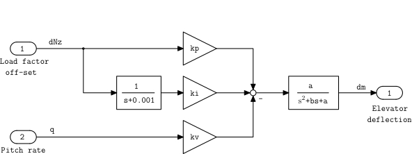
If we extract the controller from the previous figure, we can see that it consists of an
architecture with a PI controller on the load factor off-set

d N_{z}

, added to a simple gain
on input

q

, in series with a low-pass filter. Altogether

K (s)

has 5 unknown parameters,

k_{p}, k_{i}

for the PI,

k_{v}

for the gain, and

a, b

for the filter. To represent these unknowns we
use the compact notation

θ = (k_{p}, k_{i}, k_{v}, a, b) \in R^{5}

. We write

K (θ)

to indicate that

K

depends on

θ

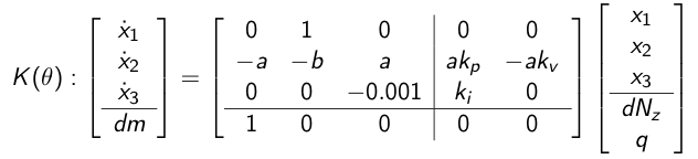
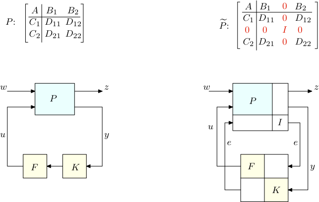
. In state-space form itcan be written as

where the unknowns

θ

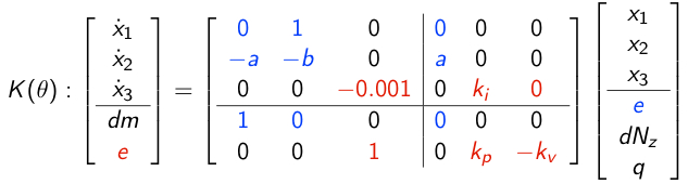
enter nonlinearly. Using a simple trick which consists in
augmenting the plant by an additional input and output,

e

, we can linearize this
controller to obtain the equivalent form

As indicated by the red and blue elements, this leads to a decentralized structure.
In the plant the linearization requires the following operation, which replaces the
two elements in series by a single now decentralized controller.

The H∞ control problem is solved

by

Pierre Apkarian and Dominikus Noll

The H_∞ control problem is solved