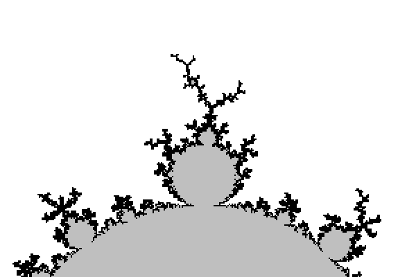
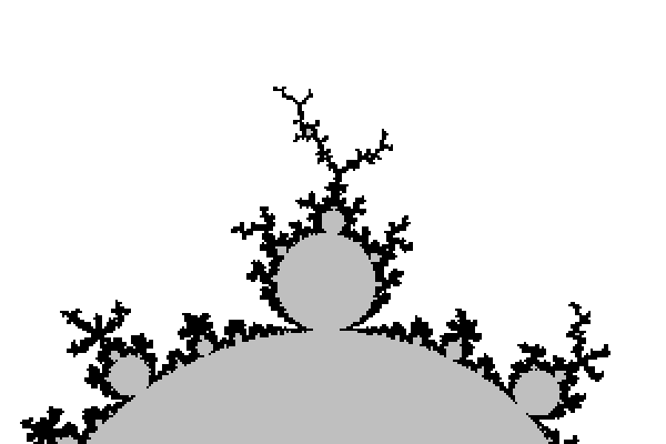
Mandelbrot set
Here we will give a few algorithms and show the corresponding results.
Contents
The Mandelbrot set
Certainly, Wikipedia's page about this set in any language should be a good introduction. Here I give a very quick definition/reminder:
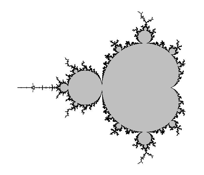
The Mandelbrot set, denoted M, is the set of complex numbers $c$ such that the critical point $z=0$ of the polynomial $P(z)=z^2+c$ has an orbit that is not attracted to infinity. If you do not know any of the italicized words, go and look on the Internet.
It is significant for two reasons:
- The Julia set of $P$ is connected if and only if $c\in M$.
- The dynamical system $z\mapsto P(z)$ is stable under a perturbation of $P$ if and only if $c\in \partial M$, where $\partial $ is a notation for the topological boundary.
Bibliography
Methods presented here are either direct translation or enhancement of algorithms that I learned first in the 1980's from elementary programs found in popular journals about computers, in the mid 1990's in the book The beauty of Fractals, and then when I started a career as a mathematician in the late 1990's directly from discussion with colleagues, especially Xavier Buff, Christian Henriksen and John H. Hubbard.
A major proportion of the main ideas and algorithms are already present in The science of Fractal Images.
The Mu-Ency by Robert Munafo contains a more detailed discussion of some of the algorithms.
- Peitgen, Richter, The beauty of Fractals, 1986, Springer-Verlag, Heidelberg.
- Peitgen, Saupe (Editors), The Science of Fractal Images, 1987, Springer-Verlag.
- Mu-Ency - The Encyclopedia of the Mandelbrot Set, 1996-2016 Robert P. Munafo.
- wikibooks.org: Fractals
Drawing algorithms
All the algorithms I will present here are scanline methods.
Basic algorithm
The most basic is the following, it is based on the following theorem:
Theorem: The orbit of 0 tends to infinity if and only if at some point it has modulus >2.
This theorem is specific to $z\mapsto z^2+c$, but can be adapted to other families of polynomials by changing the threshold $2$ to another one. Here the threshold does not depend $c$ but in other families it may.
Now here is the algorithm:
Choose a maximal iteration number N
For each pixel p of the image:
  Let c be the complex number represented by p
  Let z be a complex variable
  Set z to 0
  Do the following N times:
    If |z|>2 then color the pixel white, end this loop prematurely, go to the next pixel
    Otherwise replace z by z*z+c
  If the loop above reached its natural end: color the pixel p in black
  Go to the next pixel
I am not going to use the syntax above again, since it is too detailed. Let us see what it gives in a Python-like style:
for p in allpixels: # replace here by your own loop or pair of loops to scan all pixels
  c = p.affix # here you may replace by your code computing c (complex nb)
  z = 0j
  color = black # 'color' will be assigned to p at the end, black is a temporary value
  for n in range(0,N):
    if squared_modulus(z)>4:
      color = white
      break # this will break the innermost for loop and jump just after (two lines below)
    z = z*z+c
  p.color = color # so it will be black unless we ran into the line color=white
Note that if $z=x+iy$ then its squared modulus is $x^2+y^2$ whereas $|z|=\sqrt{x^2+y^2}$. Not only working with squared_modulus saves one step: taking a square root, but also this step is usually a time consuming one.
Here in a C++ like style: (std::complex<double> simplified into complex)
for(int i=0; i<height; i++) {
  for(int j=0; j<width; j++) {
    complex c = some formula of i and j;
    complex z = 0.;
    for(int n=0; n<N; n++) {
      if(squared_modulus(z)>4) {
        image[i][j]=black;
        goto label;
      }
      z = z*z+c;
    }
    image[i][j]=white;
    label: {}
  }
}
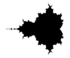
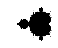
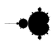
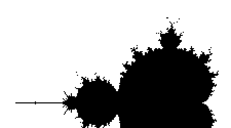
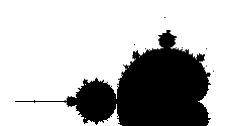
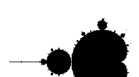
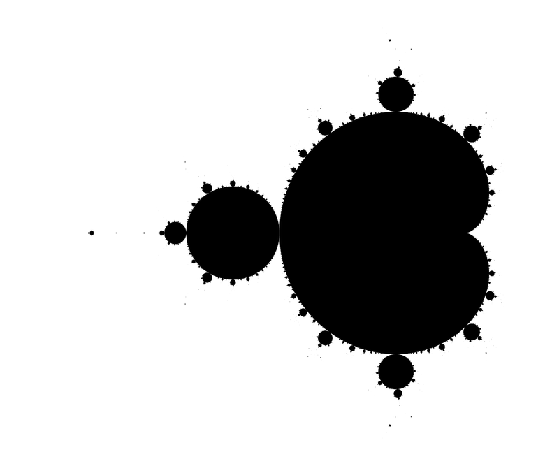
Let us now look at the kind of pictures we get with that. We took an image size of 241×201 pixels, with a mathematical width of 3.0 and so that the center pixel has affix -0.75. The only varying parameter between them is the maximal number of iterations N.
All images except the last one took a fraction of a second to compute on a modern laptop. Back then in the 1980's it was different.
Ideally the maximal number of iterations N should be infinity, but then the computation would never stop. The idea is then that the bigger N is, the more accurate the picture should be.
The N=one million image took 45s to compute on the same laptop, which is pretty long given today's computers power. What happens? Every black pixel requires $10^6$ iterations, and since there are 9 771 of them, we do at least ~$10^{10}$ times the computation z*z+c. To accelerate this, one should find a way to detect that we are in M so that we use less than the maximal number of iterations.
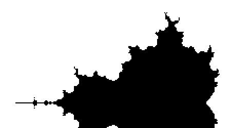
But that is not the only problem with increasing N. Not only it took much time, but the difference with N=100 is pretty small. Worse: it seems that by increasing N we are losing parts of the picture. What happens is that we are testing pixel centers or corners, and there are strands of M that are thin and wiggle between the pixel centers, so that as soon as N is big enough, the pixel gets colored white.
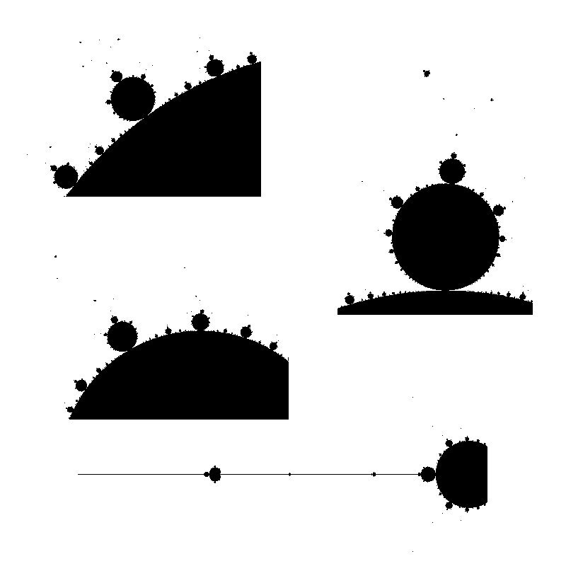
Here are enlarged versions of parts of these images, so that pixels are visible.
Let us look at a parts of a higher resolution image, computed with a big value of N: notice the small islands. The set M is connected in fact, but the strands connecting the different black parts are invisible, except some horizontal line that appears because, by coincidence, we are testing there complex numbers that belong to the real line: $M\cap \mathbb{R} = [-2,0.25]$.
The next image has been computed using a 4801×4001px image and then downscaling by a factor of 6 (in both directions) to get an antialiased grayscale image. It also has been cropped down a little bit, to fit in this column without further rescaling.
Last, an enlargment to see the pixels of the above image:
Escape time based coloring
There is a simple and surprisingly efficient modification of the above algorithm.
We started from z=0 and iterated the substitution $z\mapsto z^2+c$ until either |z|>2 (the orbit escapes) or the number of iterations became too big. Instead of coloring white the pixels for which the orbit escapes, we assign a color that depends on n, the first iteration number for which |z|>2.
def f(n): # this function returns a color depending on an integer n
  return ... # put here your custom code
for p in allpixels:
  c = p.affix
  z = 0j
  color = black
  for n in range(0,N):
    if squared_modulus(z)>4:
      color = f(n)
      break
    z = z*z+c
  p.color = color
For the coloring, you are free to take your preferred function of n, I will not develop on that here.
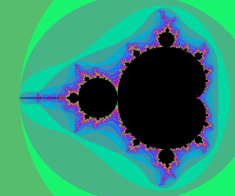
Here is an example of result:
The strands are now visible.
Here is another one, on a 4801×4001px grid, downscaled by a factor 5, with N=10000 (which is probably a bit excessive in this particular case).
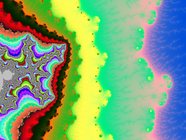
With a nicely chosen color function, one can get pretty results:
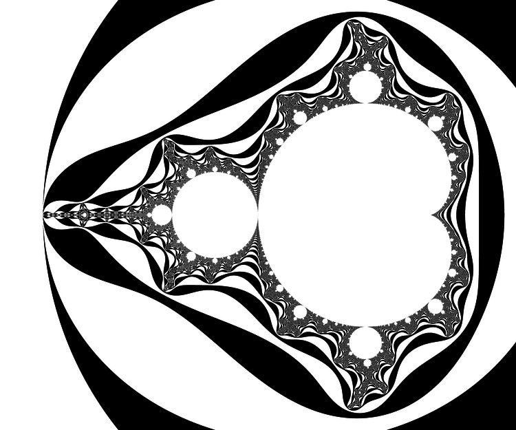
The following was popular in printed books:
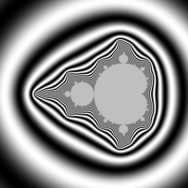
The potential
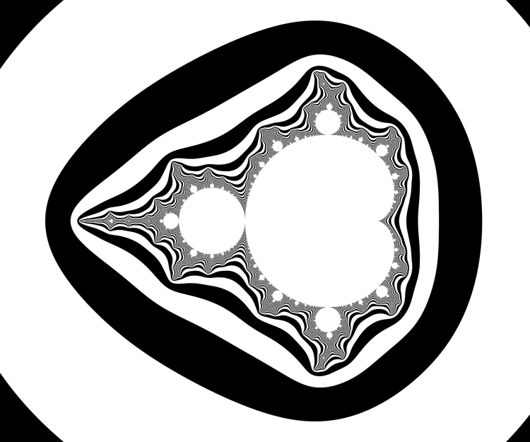
You may replace the test |z|>2 by |z|>R, provided that R>2. In fact the picture looks better that way. It has an explanation in terms of the potential.
- Physics digression: In very informal terms, in a 2D euclidean universe, put an electrostatic charge on some conducting bounded connected set K, the rest of 2D space being void (dielectric). You will put charge=-1 and assume there are so many particles (electrons) that the charge can be considered as a continuum. Then let the charges spontaneously move to minimize the energy. The resulting distribution has the property that the potential is constant on K. The potential function $V$ satisfies the Laplace equation $\Delta V=0$ outside K and $V(c)\sim \rho \log|c| $ when $|c|\longrightarrow+\infty$, for some constant $\rho$.
There is however no need to invoke electrostatics and one can define directly the following function and decide to call it the potential: $$V(c)=\lim_{n\to+\infty} \frac{\log_+|P_c^n(0)|}{2^n}$$ where $\log_+(x)$ is defined as $0$ if $x<1$ and $\log(x)$ otherwise. The exponent n in $P_c^n$ refers to composition, not exponentiation: $P^n(z)$ is P applied n times to z. The function V takes value 0 exactly on M. If x>0, the sets of equation V=x are called equipotentials of M. They foliate the outside of M into smooth simple closed curves that encircle it. The potential also finds an importance in the mathematical study of M, as holomorphic functions are involved, but that is not a the topic to be discussed here.
The fact that the formula converges and that its limit has the stated properties is not supposed to be obvious: it is a theorem too. One good thing about the formula is that it converges quite well: if we stop the iteration when |z|>R, the relative error will be of order 1/R. Now assume the picture is drawn for $|c|<10$ (anyway all points of M satisfy $|c|\leq 2$) and at some point in the iteration of $0$ we reach $|z|>4$. Then a value of $|z|>1000$ is reached pretty fast because $|P(z)|=|z^2+c|>|z|^2-5$: one sees that in 4 more iterations we have at least |z|>443556...
In the computation, when |z|=R after n iteration, and R is big enough, it means $V(c)\approx\log(R)/2^n$. Hence taking R=1000 in the previous algorithm (see the picture above) yields color regions whose boundaries very closely match the equipotentials $V(c)=\log(1000)/2^n$. This is what the picture above shows.
But we can do better: as soon as $|z|>1000$, we have a good approximation $V(c)\approx\log|z|/2^n$, and we can thus choose a continuous coloring scheme depending on $V(c)$.
Here is a possible algorithm:
def f(V): # this function returns a color depending on a float V
  return ... # put here your custom code
for p in allpixels:
  c = p.affix
  z = 0j
  color = inside_color # color may be modified below and assigned to p
  pow = 1. # pow will hold 2^n
  for n in range(0,N):
    R2 = squared_modulus(z)
    if R2>1000000: # 1000 squared
      V = log(R2)/pow
      color = f(V)
      break # this will break the innermost for loop and jump just after
    z = z*z+c
    pow = pow * 2.
  p.color = color
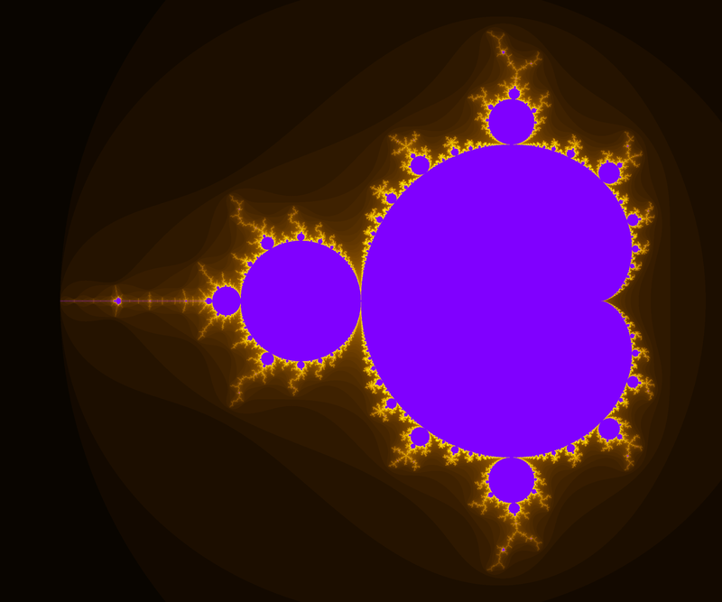
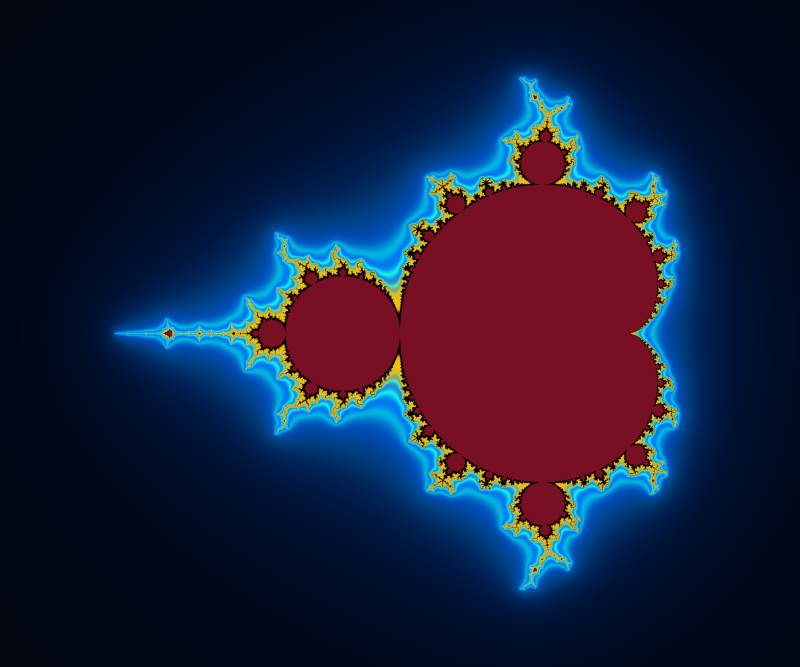
And here an example of result: computed with N=2000 and 4800×4000px and a color function that starts black away from M, then slighlty oscillate in shades of blue like a sine function of log(V), but when V gets small a uniform egg yellow color takes over, and even closer it is a black one. The set M is in dark bordeaux red.
Deep zooms and log-potential scale
The function $V$ is continuous and has value $0$ exactly on M.
The function $\log V$ is better suited than $V$ for coloring deep zooms. For instance in many points (especially tips and branch points which are asymptotically self-similar [Tan Lei]) a zoom will essentially shift the value of $\log V$ by a adding a constant that depends on the point on which you zoom.
A simple choice is to have a color that cycles when some chosen constant is added to $\log V$. This choice is also a heritage from when images had a limited palette. So choose $K>0$ and set $$x=\log(V)/K$$ $$\mathrm{color}=g(x)$$ for some function g with g(x+1)=g(x). You can enforce periodicity by reducing x modulo 1 to [0,1[ but that may introduce discontinuities if g was not 1-periodic. For instance $$g(x)=(R,G,B)=(255,255,255)\times\frac{1+\cos(2\pi x)}{2}$$ will yield a smooth wave pattern, from white to black and back.
Taking $K= \log 2$ is a good starting choice, as it is "natural" for reasons we will explain later. You may already notice that $\log \log P(z) \approx (\log\log |z|) + \log 2$ when z is big. However, M gets quite furry in some deep zooms, it is then better to divide by a bigger constant in this case.
Below, some illustrations: Instead of a periodic function we chose a quasiperiodic one: $$g(x)=(R,G,B)=\left(255\times\frac{1-\cos(a x)}{2},255\times\frac{1-\cos(b x)}{2},255\times\frac{1-\cos(c x)}{2}\right)$$ with $(a,b,c)=\left(1,\frac{1}{3\sqrt2},\frac{1}{7\cdot3^{1/8}}\right)\times\frac{1}{\log 2}$ linearly independent over $\mathbb{Z}$. (It is not the prettiest choice; this is not the point, though.)
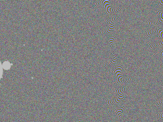
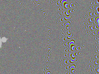
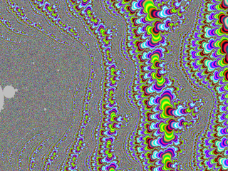
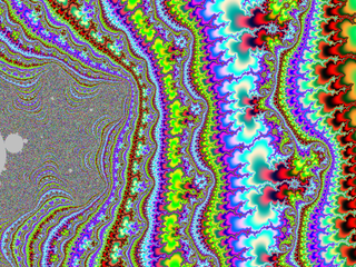
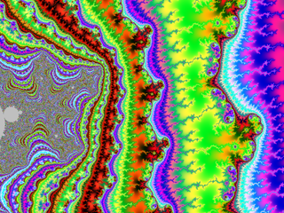
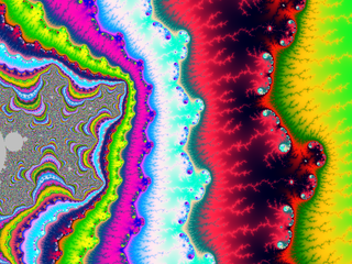
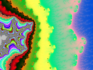
Below, 12 views of the same deep zoom on M. Only K varies, taking respective values 0.03, 0.1, 0.3, 1, 3, 10, 30, 100, 300, 1000, 3000 and 10000. They are all downscaled by a factor 2 from an original of 2400×1800px. They is a further rescaling in the thumbnails below, but you can click on them to get the 1200×900px version.
It is particularly visible on the 7th one, that not one value of K can capture all the filamental structure : on the right it is barely visible, and on the left near the circular gray shapes it is a mess.
Note: the computation of the images above have been accelerated using the interior detection method described later in this page.
Interior detection methods
Math digression: hyperbolic components
We must now introduce hyperbolic components. If you take c inside M, there is a good chance that c will belong to one.
Definitions:
- A periodic point for P is a point $a$ such that $P^k(a)=a$ for some k>0.
- The first $k>0$ for which this occurs is called the period of a.
- The orbit of $a$ is then finite: it is called a cycle.
- The value of $(P^k)'$ is the same at any point in the orbit of a: it is called the multiplier of the cycle.
- A cycle is called attracting or attractive or a sink if the multiplier has modulus<1.
- A parameter c is called hyperbolic if $P_c$ has an attracting cycle.
Recall that $P_c$ is defined by $P_c(z)=z^2+c$. For hyperbolic parameters, Fatou proved* that the critical point is attracted to this cycle. In particular, $c\in M$.
(*) This is a quite striking feature of non-locality holomorphic dynamics: the cycle has an attracting power that reaches to the critical point.
Fatou also prove that $P_c$ can have at most one attracting cycle.
Why call this "hyperbolic"? In more general dynamical systems, this word has another definition, which in our case would read as follows: $P_c$ is expanding on its Julia set. It turns out that the two definitions are equivalent, a highly non-trivial fact.
Hyperbolic parameters are stable: all nearby parameters are also hyperbolic, the attracting cycle and the Julia set move continuously when $c$ varies in a small neighborhood. The hyperbolic component associated to $c$ is the connected component of the set of hyperbolic parameters that contains c. Such a component is bounded by an algebraic curve, smooth except at at most one point. This curve is composed of those parameters for which the multiplier of the cycle has modulus one. In fact for this family $P_c$, the components are either like disks or like interior of cardioids. They have no holes.
It can be proved that these boundary curves are contained in the topological boundary of M: hence a hyperbolic component is also a connected component of the interior of M. We do not know if the converse holds: this is Fatou's conjecture, still open today:
Conjecture: All connected components of the interior of M are hyperbolic.
It is a big conjecture. Solve it and become famous.
Following the derivative
As we iterate z, we can look at the derivatives of P at z. In our case it is quite simple: $P'(z)=2z$. Multiplying all these numbers along an orbit yields the derivative at z of the composition $P^n$. This multiplication can be carried on iteratively as we iterate z:
  [...]
  der = 1
  z = c # note that we start with c instead of 0, to avoid multiplying the derivative by 0
  for n in range(0,N):
    new_z = z*z+c
    new_der = der*2*z
    z = new_z
    der = new_der
    [...]
If we started from the critical point there is a 0 at the beginning of the product, so $(P^n)'(0)=0$. However, omitting the first term yields $(P^n)'(c)$, which has a good chance to be non-zero: it will be 0 if and only if 0 is periodic, which corresponds to the centers of the hyperbolic components of M, a notion that I will not develop here: you just need to know that they lie in the smooth areas inside M.
Note: See the lines?:
    new_z = z*z+c
    new_der = der*2*z
    z = new_z
    der = new_der
It is to avoid a frequent mistake:
    z = z*z+c
    der = der*2*z
Would not work, whereas
    der = der*2*z
    z = z*z+c
would. See why?
The idea
Now if $c$ is a hyperbolic parameter then its orbit tends to an attracting cycle and therefore the derivative above will tend to $0$. The converse does not exactly hold, but the counterexample values of $c$ are sparse.
The basic idea is then to choose a threshold and stop the computation when the derivative $(P^n)'(c)$ has reached a modulus below this threshold $\epsilon$ and declare the pixel to be in M (in its interior in fact) and color it according to this and your taste.
It may wrongly mark as interior some points that are not. The hope is that the mistake is barely noticeable.
for p in allpixels:
  c = p.affix
  z = c
  der = 1+0j
  color = not_enough_iterates_color # replace it by inside_color if you prefer
  for n in range(0,N):
    if squared_modulus(der) < eps*eps: # eps is the threshold, a small number
      color = inside_color
      break    # here, this jumps to the last line
    if squared_modulus(z) > R*R:   # put here your preferred R>=2
      color = outside_color        # replace here by your preferred color scheme outside M
      break    # here, this jumps to the last line
    der = der*2*z   # order matters: do not modify z --before-- computing the new der
    z = z*z+c       # order matters
  p.color=color # last line
This method was first explained to me by Xavier Buff, who tested it and told me it gives good result, which I never would have thought.
So, does criterion work? Does getting below $\epsilon$ ensure that there is an attracting periodic cycle ? What would be the danger? The orbit of $c$ could spend too much time in the area where $|P'|<1$, or it may pass a few times too close to $0$. In the second case it seems intuitive that $c$ must be close to the center of a hyperbolic component. But what about the first case?
In fact there are some well chosen non-hyperbolic values of $c$ such that $\liminf_n (P^n)'(c) =0$, but these are very rare. Moreover, any point outside M will satisfy $\inf (P^n)'(c) \geq f(V(c))$ for some function $f>0$, thus at least the points detected by the method that are not in M are close to M, and this distance can be made small by decreasing the threshold.
Images and speed
In short:
The improvement in speed is not so impressive in the case of M. However the usefulness of the interior detection method appears elsewhere: to get a comparable computation time without it, one has to fine-tune the maximal number of iterations N; when you zoom this has to be adapted by hand. With the method you can save this pain: you can start with a too big value, it makes little difference in the computation time.
Let us be more precise:
Notice that each iteration of the new method requires twice the amount of computations as an iteration with the old method (the ratio may be closer to 1 with more elaborate families and/or algorithms). Even if the interior of M covers a big part of the picture, there seems to be a well-chosen value of $N$ such that the average number of iterates necessary to reach a given accuracy with the old method is no more than 3 times than with the new method. So the computation time is only divided by 1.5.
There is nevertheless another aspect for which the interior detection trick has a clear advantage. You can use a too big N even at low zoom factors ($N=10^6$ is OK, but avoid N=$10^{10}$), it will barely make a difference because most points will stop much earlier anyway. This number N will work for a bigger range of zoom factors before you have to increase it.
Below, a simple experiment:
It is quite surprising that a not-so-small value of epsilon gives a pretty good image of M. The problems seem to concentrate at parabolic parameters. Below a zoom near c=-3/4, with epsilon=1/10, enlarged to make pixels visible.
Boundary detection methods via distance estimators
Milnor's
The first distance estimator method that I learned of was taught to me by Douady, it seems to be due to Milnor and Thurston, see [1],[2].
Principle
If $0$ escapes under the iteration of $P:z\mapsto z^2+c$, let $z_0=0$ and $\rho_n = dz_n/dc$. Choose a threshold $R>2$ big enough (for instance $R=1000$). Choose an $n$ such that $|z_n|>R$. An approximation of the distance from $z$ to $M$ is then given by the quantity $$d_n=\frac{2|z_n|\log|z_n|}{\rho_n}.$$
The sequence $\rho_n$ can be computed iteratively along with $z_n$: $\rho_0=0$ and $$\rho_{n+1}=2 z_n \rho_n + 1$$
Note: This is a bit analogous to the computation done in Section Following the derivative, with one important difference: we compute $\displaystyle\frac{dP_c^n(c)}{dc}$, not $\displaystyle\frac{dP_c^n(z)}{dz}$ (where $c$ would be constant); the resulting inductive formula is thus different.
[insert example with formula wrong]
Caution: It is not true that this approximation $d_n$ tends to the actual distance $d$ from $z$ to $M$ when $n$ tends to infinity. In fact, only weaker inequalities hold: $d_n$ converges and $1/5<d/\lim d_n<1$ provided $|z|<5.7$. The lower bound 1/5 can be replaced by a function that depends on $|z|$, but can never be better than 1/4. If $R=1000$ and $|z_n|>R$, then $d_n$ is pretty close to $\lim d_n$.
Math
The math behind the method has a higher level of sophistication. It is based on the following:
- A conformal map from the outside of $M$ to $U$, the outside of the (closed) unit disk, is known: this is $c\mapsto\phi_c(c)$, where $\phi_c$ is the conformal map from the outside of the filled-in Julia set to $U$.
- A simple and efficient way of estimating $|\phi_c(c)|$ and $|\partial\phi_c(c)/\partial c|$.
- Conformal maps respect the hyperbolic metric.
- A correlation between the hyperbolic metric coefficient and the Euclidean distance to the boundary.
Let me give a few more comments on that, though I won't explain the whole thing. First, the infinitesimal expression of a hyperbolic metric takes the form $\rho(z)|dz|$ where $\rho(z)>0$ (such expressions are called conformal metrics). Then, the hyperbolic metric on $U$ has the following infinitesimal expression: $|dz|/(2|z|\log|z|)$. Concerning the 3rd point, if $f$ is holomorphic, then the image of this metric by $f^{-1}$ has expression $|f'(z)|\rho(f(z))|dz|$. Concerning the 4th point above, if we were dealing with a simply connected set (which we aren't) then there is a very nice theorem : on a simply connected open subset $O$ of the complex plane, the coefficient $\rho$ of the hyperbolic metric $\rho(z)|dz|$ lies between $1/d$ and $4/d$ where $d$ is the distance from $z$ to the boundary of $O$. I think the idea in the method above is that it remains nearly true: other estimates, close to this one, can be given. I have not tried to figure out a nice and correct estimate so I'm not giving one here.
Implementation
Note: Don't forget in your program to: either modify $\rho_n$ before $z_n$; or better, store the new values of $\rho$ and $z$ in temporary variables and only after assign them to $\rho$ and $z$. The algorithm should look like that:
thickness_factor = 1. # change this if you want to tune the boundary thickness

for p in allpixels:
  c = p.affix
  z = c
  der_c = 1+0j # this is the derivative w.r.t c
  reason = NOT_ENOUGH_ITERATES

  for n in range(0,N):
    if squared_modulus(z) > R*R:
      reason = OUTSIDE
      break
    new_z = z*z+c
    new_der_c = der_c*2*z + 1   # notice the difference with the formula for the z-derivative
    z = new_z
    der_c = new_der_c
  # the break above jumps here

  if reason == NOT_ENOUGH_ITERATES:
    p.color = not_enough_iterates_color
  else: # in this case reason = OUTSIDE
    rsq = squared_modulus(z)
    # the test below is equivalent to testing d_n < thickness_factor*pixel_size
    # d_n is defined in the text above this code snippet
    # x**y means x to the power y
    if rsq*(log(rsq)**2) < squared_modulus(thickness_factor*pixel_size*der_c) :
      p.color = boundary_color
    else:
      p.color = outside_color
Note that our test d_n < thickness_factor*pixel_size is done at the level of squares, as a mild way to save computation time. It can be further optimized. However, it does not save much because most of the time is spent in the inner loop.
Result:
Comparison (zoomed) :
