DASSFLOW

Inferences of discharge, bathymetry and flow models parametrization

Simulations at watershed scale with local zooms, flood plain dynamics

Below are presented some capabilities (more or less recent...) of DassFlow software (1D and 2D shallow flow models).

Update. DassFlow is now part of DassHydro (Data Assimilation for Hydrology) plateform.
DassHydro includes DassFlow and SMASH (INRAe et al.) thus providing a complete computational plateform dedicated to hydrology (floods, inundations).
DassFlow and SMASH are built following the same technologies: Fortran kernel codes, Python wrapping, providing Data Assimilation capabilities.

*
The recent DassFlow results rely on a collaboration between INSA Toulouse / IMT (J. Monnier et al., math. modeling-comput. sc.), INRAE (P.-A. Garambois et al., hydrology modeling), CNES-CS group (K. Larnier et al., Senior Research Engineer, programming-assessing-datasets), with great PhD students and engineers: L. Villeneuve, L. Pujol, T. Malou, J. Verley and P. Brisset (IMT-INRAe-INSA-Univ. Strasbourg-CNES-CLS group). See publications' list.
Moreover the H2iVDI algorithm (K. Larnier, J. Monnier) aiming at estimating river discharges from SWOT data only (forthcoming space mission NASA-CNES et al.) is illustrated.
You can see similar colorful examples on the SWOT mission website (NASA-CNES).

The H2iVDI (Hybrid Hierarchical Variational Discharge Inference) algorithm dedicated to spatial hydrology

The computations aim at estimating the river discharge from altimetry measurements of the water surface only (forthcoming SWOT mission, NASA-CNES). The same computations can be applied to numerous rivers worldwide, see Fig. below.

Rivers that could observed by the SWOT instrument
Figure. (L) SWOT mission (launch 2021, NASA-CNES). (R) Number of reaches (~10 km long) potentially observed by SWOT instrument: the SWORD database from [Alteneau-Pavelsky et al. (2021)]. (SWOT Science Team).

The test river presented below is the Garonne river right next to our offices. A portion between Toulouse and Malause (dataset provided by IMFT, D. Dartus, H. Roux et al.). Another illustration is presented on a portion of the Sacramento River (California, USA; dataset provided by M. Durand, Ohio State Univ.).

You can consult short notes on the SWOT blog too (not recent anymore...): On Variational Data Assimilation of SWOT-like data in 1D and 2D river flow models (april 2016). See also initial thoughs: On variational sensitivities, data assimilation and inversion for small scale river flows (nov. 2013).

DassFlow 1D dedicated to spatial hydrology (combined with H2iVDI algorithm)

DassFlow 1D solves: a) the 1D SW model (Saint-Venant's equations) in variables (S,Q) using either an innovative low Froude finite volume schemes (1st or 2nd order) or the standard Priessmann's scheme; b) the diffusive wave equations (standard version and double scale version) using FE scheme.
River geometry are described by cross-sections based on trapezium superimpositions (description consistent with altimetry measurements).

The identified/control parameters are the upstream discharge (time series), the friction coefficient K (Manning-Strckler, potentially varying), the bed elevation (effective bathymetry). Potentially it is the downstream rating curve and the initial condition too.

A test river next to Toulouse: Garonne river

The considered Garonne river portion is between Toulouse and Maulause. The 1158 computational cross-sections derive from a linear interpolation between the measured cross-sections and LIDAR information in the flood plain (5 m accuracy). Datasets prepared by Fluid Mech. Institute (IMFT) Toulouse.

Figure. Left: Cross-section locations in the 1D model (Garonne river). Right: cross-section example (1D model). Dataset prepared by IMFT.

SWOT measurements

SWOT-like observations are simulated using the SWOT simulator (co-developed at LEGOS by S. Biancamaria et al.). The SWOT like observations are given by SWOT-Band of 200 m (On Fig. they are averaged at 1km scale). These SWOT observations are not synchronous: each overpass provides 2 swaths, 60km width each. Each swath is splitted into 200m width bands. Each band corresponds to a single water elevation measurement (accuracy ~ +/- 30 cm).

SWOT observation localisation
Figure 3: SWOT observation locations (asynchronous water elevation bands). Dataset prepared by LEGOS et al.

Estimation of the river bathymetry and the discharge

1 day revisiting period case (CalVal satellite phase)

The Variationa Data Assimilation process implemented into DassFlow enables to identify the triplet (Qin(t); b(x), K(h)), that is the inflow discharge, an effective bathymetry b(x) and the corresponding varying friction coefficient K(h) (h denotes the water depth).
Below are presented the computed estimations in the case of a 1 day revisiting satellite corresponding to the CalVal orbit period.

Bathymetry identified by DassFlow1D Inflow disharge identified by DassFlow1D
Figure: Garonne river (Toulouse-Malause portion), Cal-Val satellite period (1 day repeat). (L) The effective true bathymetry.
(Middle) The estimated bathymetry (the mean slope has been substracted). The prior value is obtained by a low complexity model inversion.
(R) Inflow discharge: the target value and the identified value. Case of 1 day revisiting satellite (CalVal orbit period).
Computations INSA-IMT-ICUBE-CNES-CS Group 2018.

Obviously once the flow dynamic model has been calibrated as shown above, all the river properties can be computed at any location and any instant, in particular the discharge Q(x,t). However the altimetry data make possible to accurately estimate the discharge at the ~ hours observation instants only.

An other example with ~21 days revisiting period (nominal satellite phase)
The considered river is the Sacramento river, California. The dataset has been provided by M. Durand et al. (Ohio State Univ., USA).

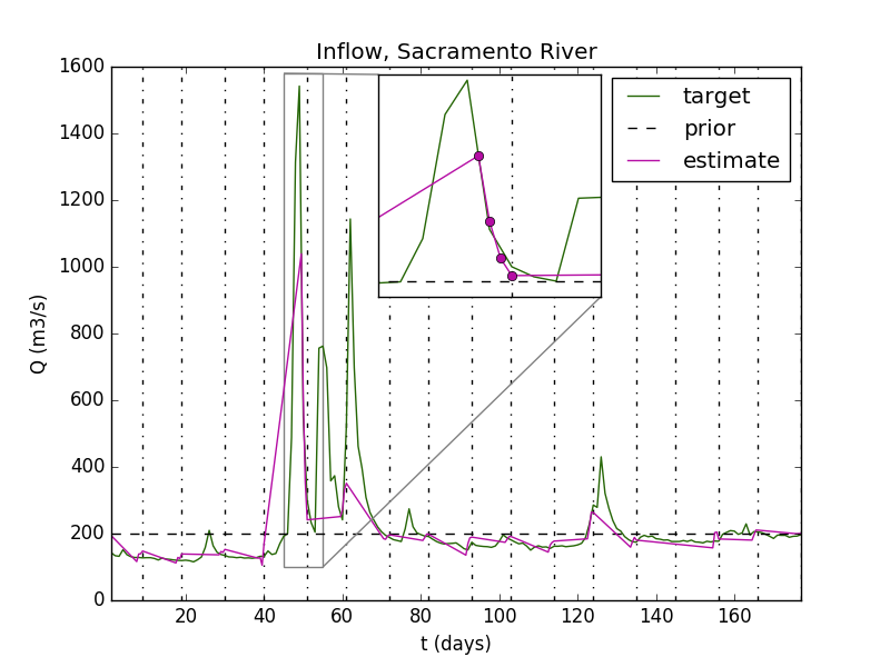
Figure: Sacramento river, estimation of the discharge from SWOT data only (data generated by the Nasa-Cnes SWOT simulator).
Computations INSA-IMT-ICUBE-CNES-CS Group 2018.

As mentioned above, the altimetry data make possible to accurately estimate the discharge, but at the hours observation instants only.

DassFlow2D for networks and local floodplains, coupled with hydrological model(s)

The forward model is based on the 2D SW equations, solved by a Finite Volume schemes (either first or second order). The conservative variables are the water depth h and the local discharge q = hu, where u = (u,v) is the depth-averaged velocity field.
The 2D solver can be degenerated in a consistant way onto a 1D solver, thus enabling lighter computatiosn and river networks modeling.
The 2D solver is used as zooms eg at branches junctions or in local flood plains.

A few examples are presented below.

Adour watershed (south-west of France).

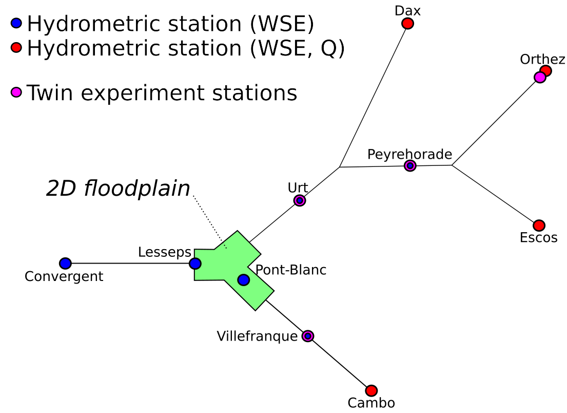
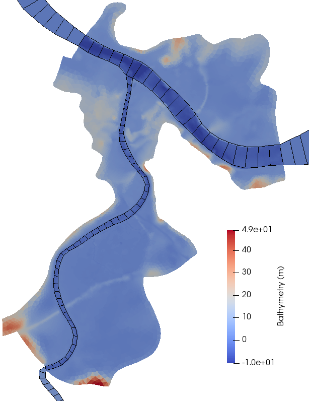
Fig. Adour rivershed (southwestern France) modeled by DassFlow2D. 1D network flows (Left) with 2D local zooms (Right), coupled with hydrological model (red points) (GR4 model from INRAe).
Datasets provided by SPC GAD. Computations Univ. Strasbourg - ICUBE L. Pujol et al.

Garonne river (south-west of France). This is the same river portion as those considered in the HiVDI algorithm presentation.
The 2D mesh cointains 436 264 nodes, 867 498 cells. The flood plain topography data derives from LIDAR + STRM information. Datasets have been post-treated by IMFT Toulouse (D. Dartus et al.).

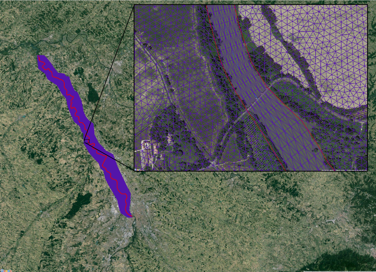
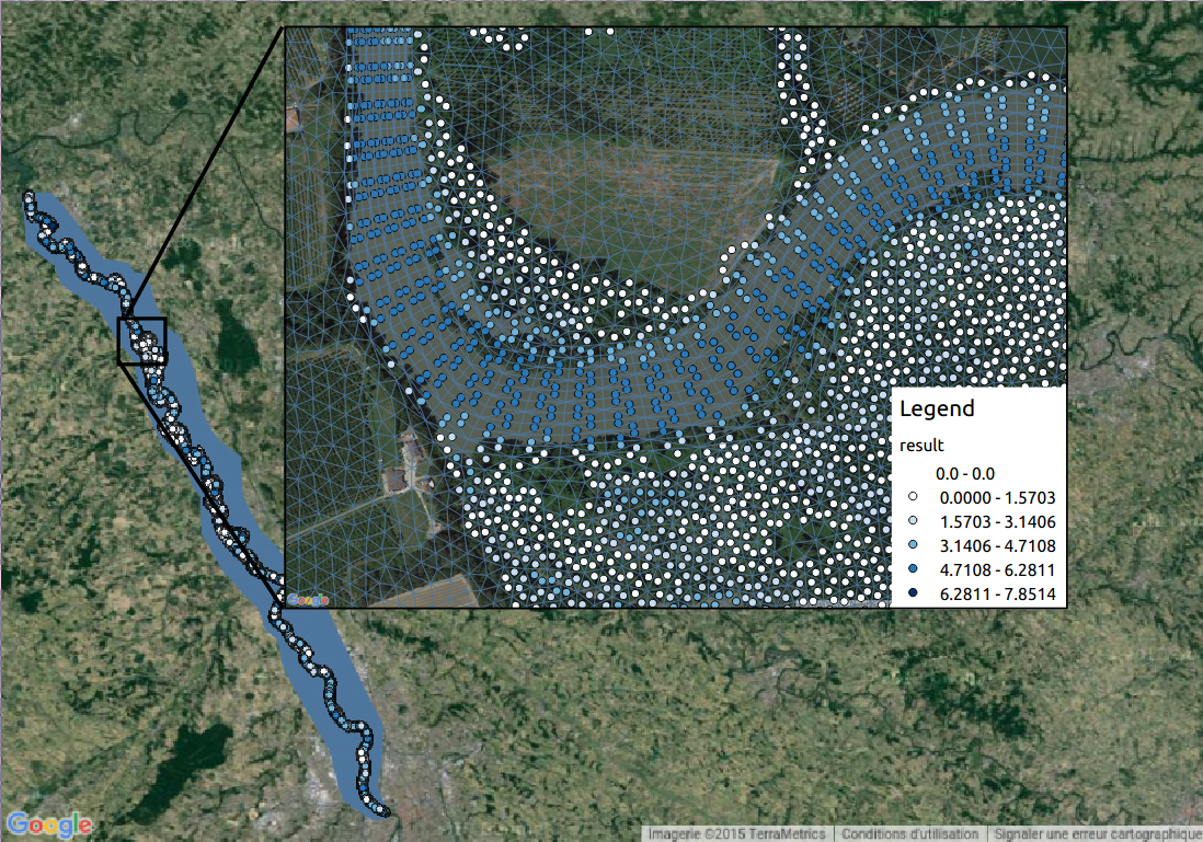
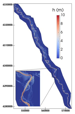
Fig. Garonne river (Toulouse-Malause portion) modeled by DassFlow2D. 867 498 cells (MPI computations both for the direct and the adjoint codes).
Dataset prepared by IMFT et al. Computations INSA-IMT-IMFT.

On the Fig. above, the flow is computed with the upstream discharge equal to 160 m3.s-1 in the common regime case and 800 m3.s-1 during the 2000 flooding event. This direct run has been used to generate SWOT-like data (synthetic data in view to twin inversion experiments).